Normal Distribution

Continuous Random Variables

• Unlike discrete random variables, continuous random variables can assume infinitely many values that correspond to points on an interval.
• Therefore, we often a different approach to generate a probability distribution for continuous random variables.

The Normal Distribution

• When graphing the probability distribution of a continuous random variable, it often results in a smooth curve.
• This smooth curve is also known as the probability density function (PDF).
  • When a continuous random variable follows a bell-shaped probability curve, it is called as the normal random variable, or it follows a normal distribution.

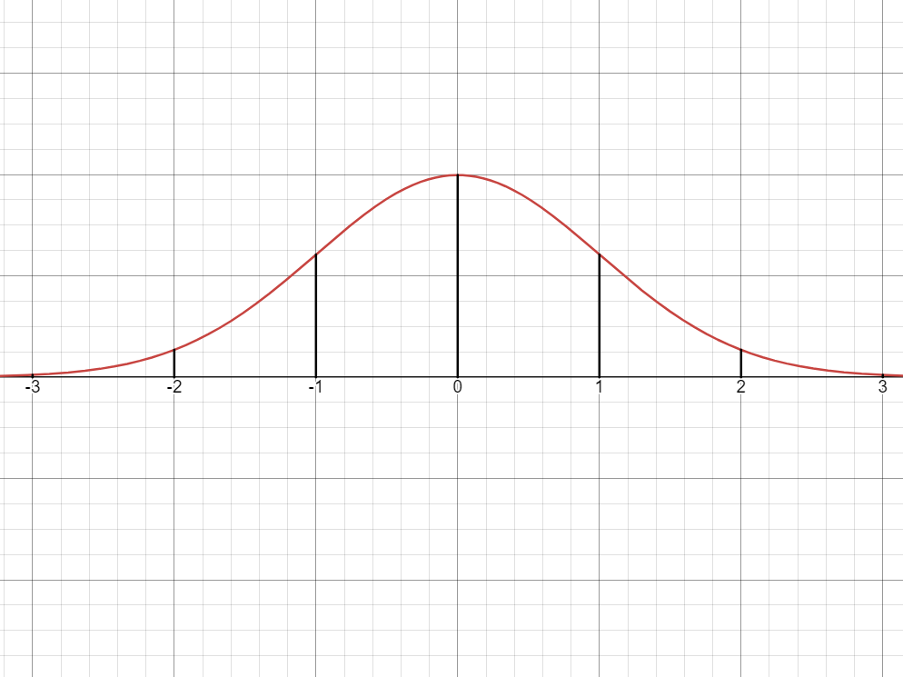
Characteristics of a Normal Distribution

• The normal distribution follows a bell-shaped curve.
• The mean, median and mode are equal.
  • They are located at the center of the distribution.
• A normal distribution is unimodal (has one mode).
• The curve is symmetric to the mean.
• The total area under the curve is .
• The curve is asymptotic to the -axis.

Using the Standard Normal Distribution

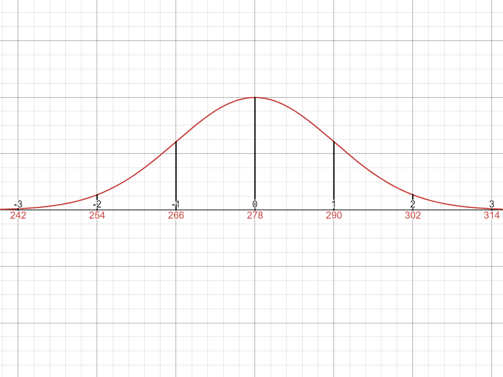
• Different sets of data correspond to different curves with different means and standard deviations.
• In that case, to simplify calculation, we convert a normal distribution to a standard normal distribution using a standard scale called the -score.
  • In a standard normal distribution, one unit corresponds to exactly units from the mean.
  • This means that if a normal distribution has a mean and a standard deviation of , then each unit in the standard normal distribution corresponds to units in the normal distribution

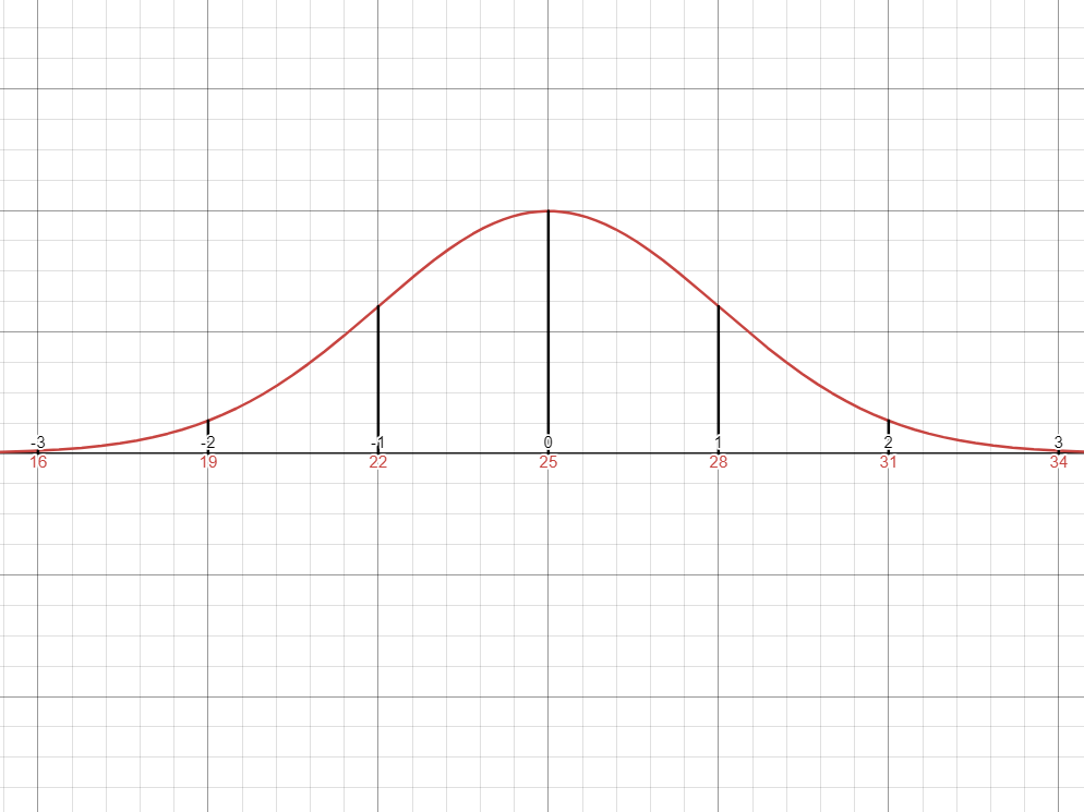
Problem

A normal distribution has a mean and a standard deviation of .
Construct a standard normal distribution that best represents this probability distribution.

Solution

Using the Standard Units

-scores

• The -scores or the standard units define the position of a score in relation to the mean using the standard deviation as a unit of measurement
• It is the number of standard deviations by which the score deviates from the mean.
  • This allows us to standardize the distributions.
• The -score of a data point is found using the formula:

where:

• data point
• population mean
• standard deviation of the population

Problem

In a population of reading scores, the mean is and the standard deviation is . Find the -value that best corresponds to a score of .

Solution

We simply use the -score formula to find its corresponding -value.

Therefore, the raw score of corresponds to a -score of .

The Standard Normal Table

• In continuous random variables, the area of a region under the bell curve corresponds to the probability of an event.
• For a normal distribution, we use the standard normal table to compute the probability of an event.

The Standard Normal Table

• It is a table of areas from the standard normal distribution.
• An entry in a standard normal table gives the area under the curve between the mean and standard deviations above the mean.

Shown below is the standard normal table for values between and

Computing Probabilities in a Normal Distribution

To compute the probability in a normal distribution, you should know some of these ideas:

• The area under the curve for the entire interval is always equal to .
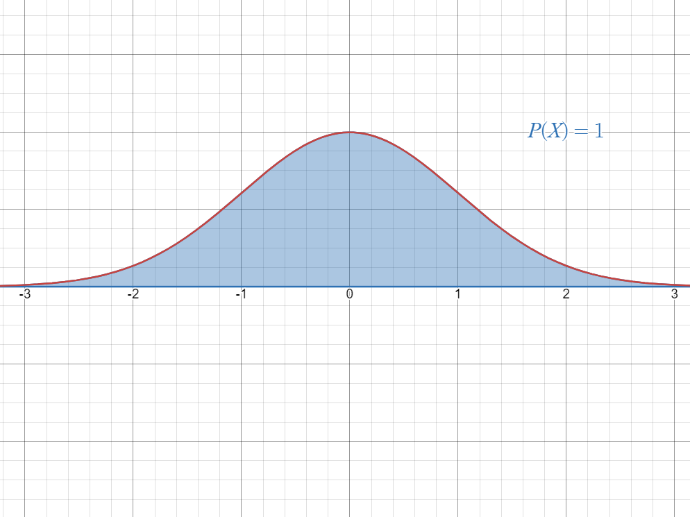
• The mean divides the curve in half.
  This means that the area to the left and to the right of the mean is always .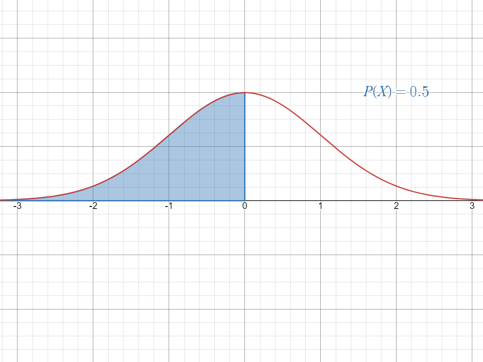
  
• Finally, the area between and is the value of in the standard normal table.
  

Problem

Find the probability of the following events:

1. Solution

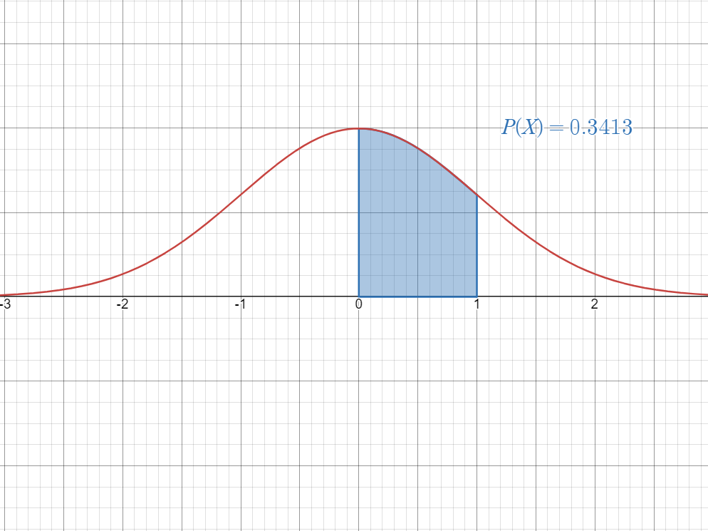
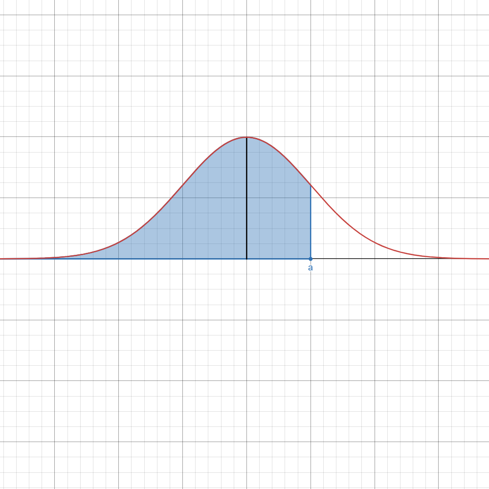
   Step 1: First, visualize the probability as an area under the bell curve.
   

   Since it is an area between and , we simply look up in the -table for the value of .

   Therefore,
   

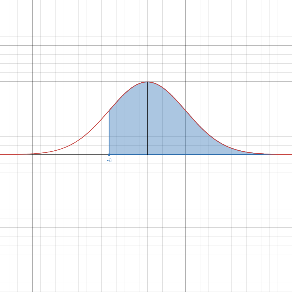
2. Solution

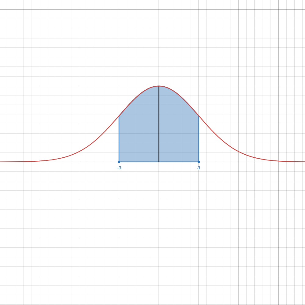
   Step 1: Visualize the probability as an area under the bell curve.
   

   Remember that a bell curve is symmetric about the mean. Therefore, it is the same as looking up the value of in the -table.

   Therefore:

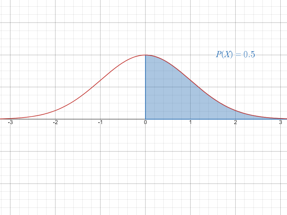
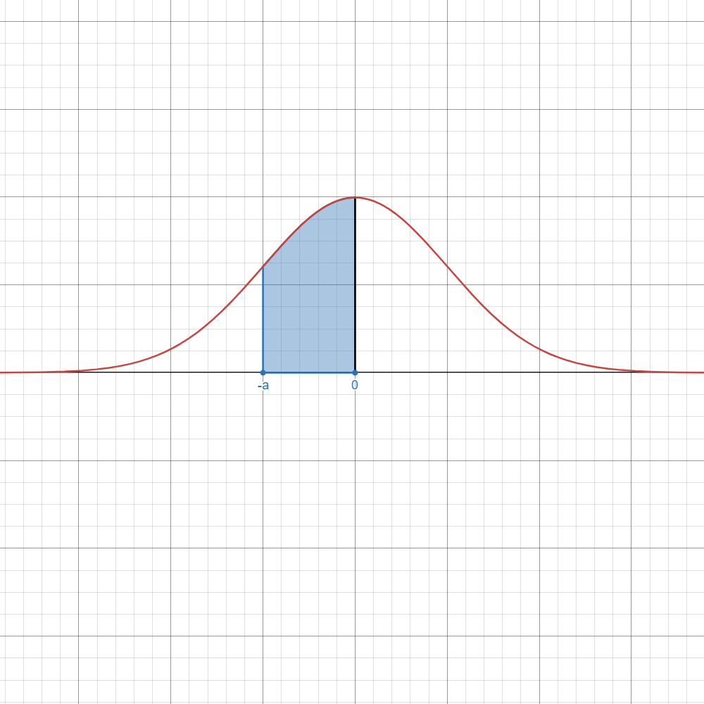
3. Solution

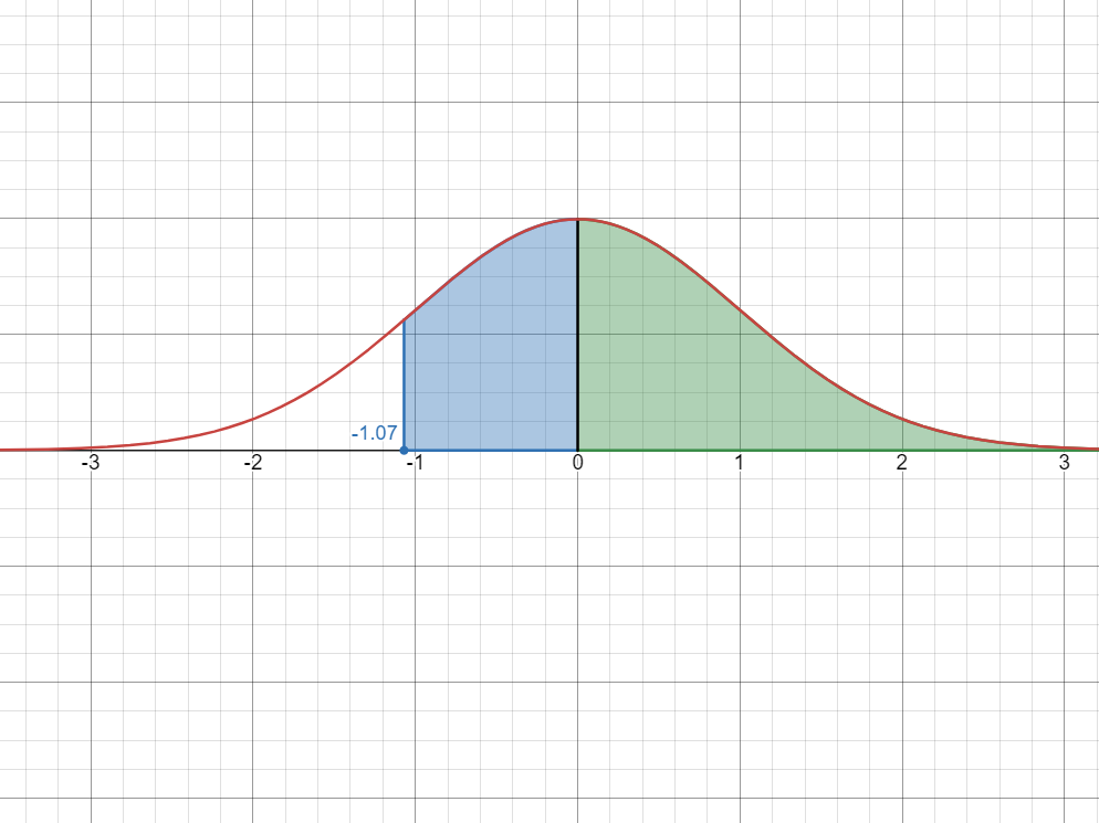
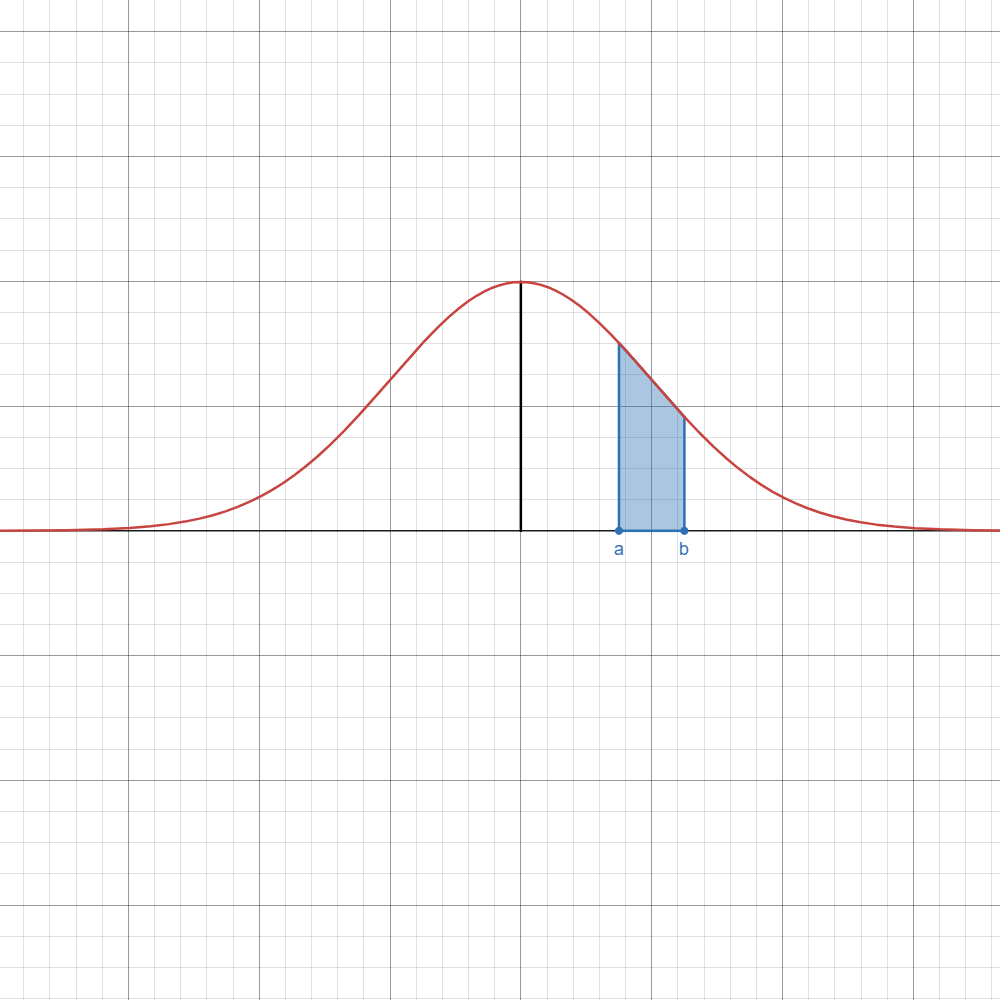
   Step 1: Visualize the probability as an area under the bell curve.
   

   Looking at it, it doesn’t seem like we can compute its probability. However, what we can do is divide the area itself into smaller parts.

   Step 2: Divide the area
   

   Now, we can see that we can divide the area in two parts, one covering the half of the curve (in green), and one between and .

   • We know how to compute the blue area from to : this is the same as finding in the -table, which gives us .
   • Since the other half (green area) is fully covered, we know that its probability is exactly , therefore:

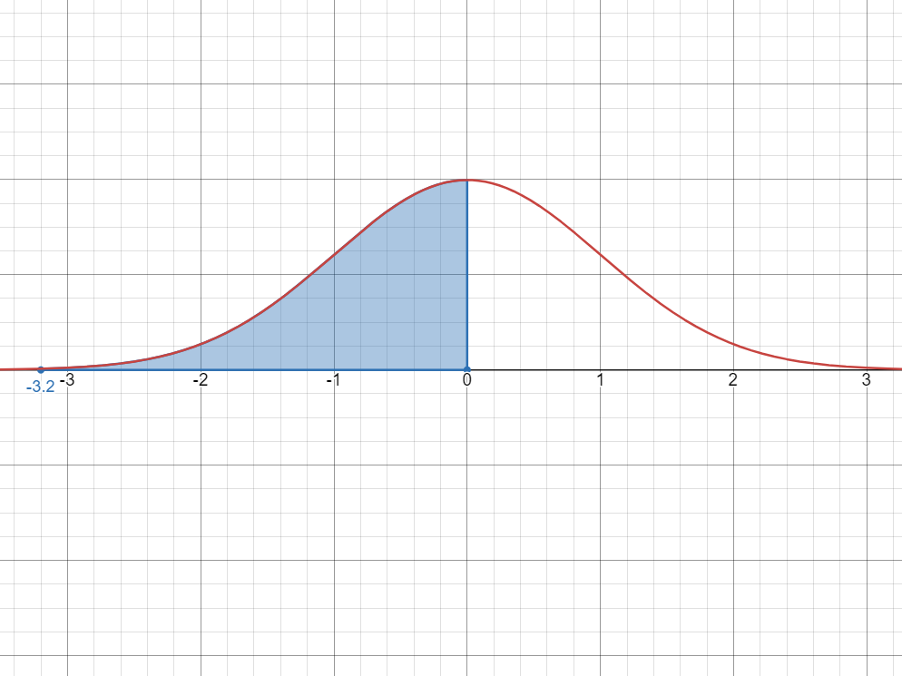
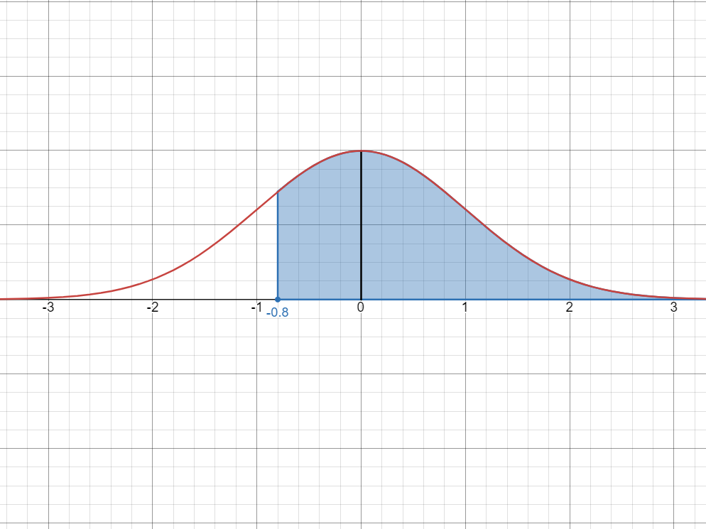
4. Solution

   Step 1: Visualize the probability as an area under the bell curve.
   

   Again, we should see if there’s some way if we could divide the areas again.

   Step 2: Divide the areas
   

   We see here that if we consider the green area, the areas add up to a half of the curve .

   Therefore, to get the blue area, we can simply subtract the green area to .

   • Since the green area is the area between 0 and , we simply have to look for in the -table, which is

   Therefore:

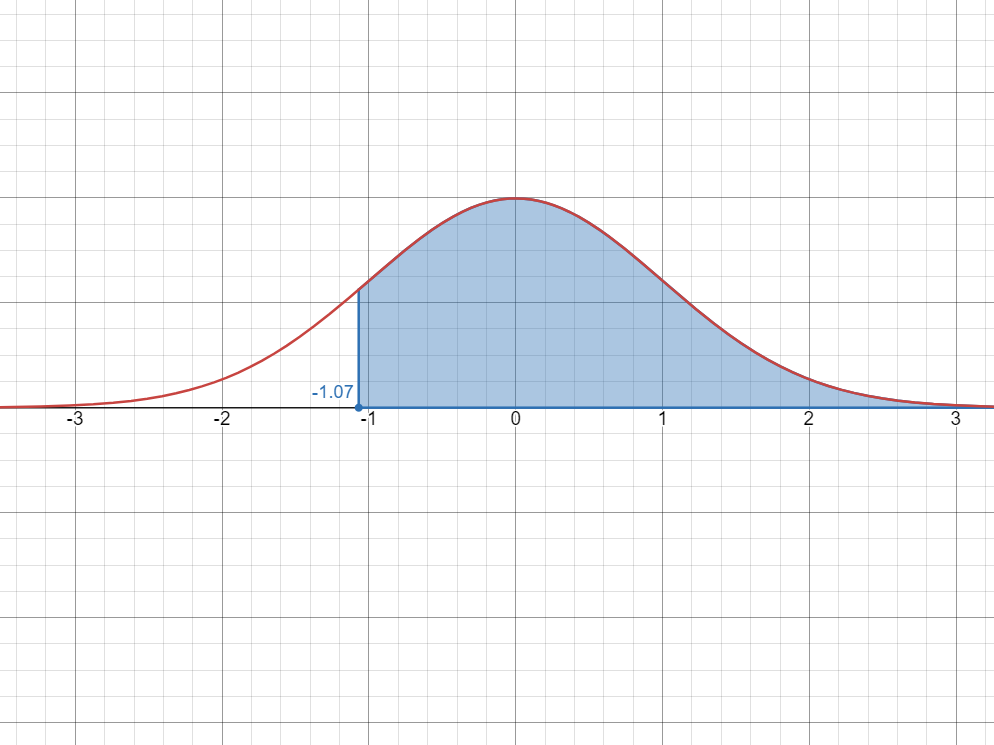
5. Solution

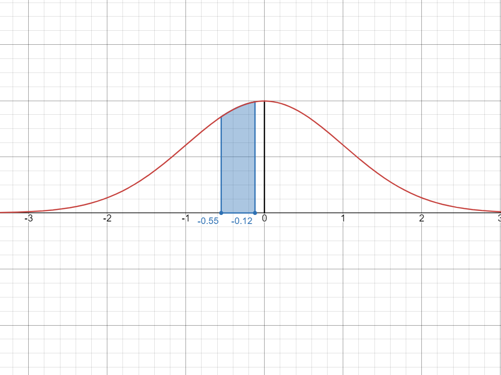
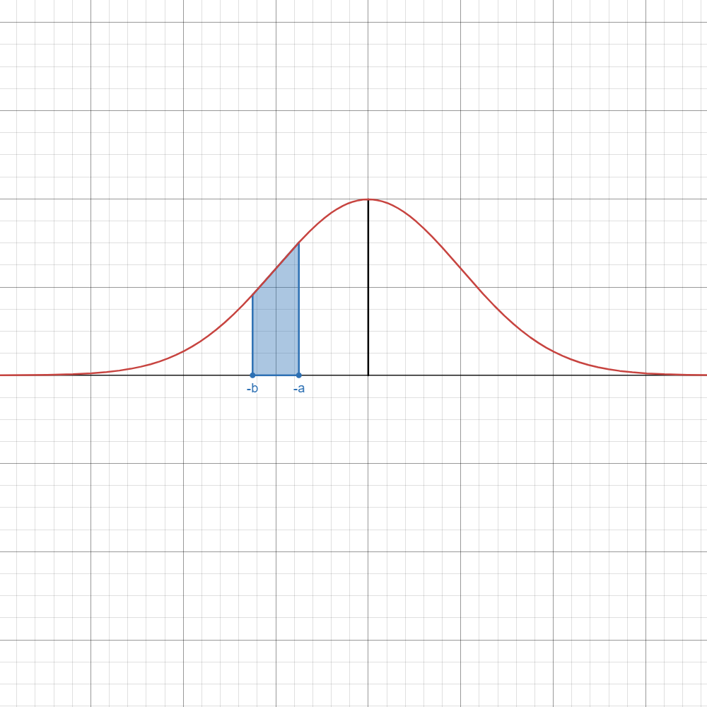
   Step 1: Visualize the probability as an area under the bell curve.
   

   Again, we can reason out by thinking how can we divide the area to compute the probability.

   Step 2: Divide the area
   

   One strategy is to compute the larger area, then subtract the red area from the blue area.

   • The blue area is the area from to , which is the same as looking up in the -table, which gives us

   • The red area is the area from to , which is the same as looking up in the -table, which gives us

     Therefore:

P(-0.55 < X < -0.12) = 0.2088 - 0.0478 = 0.161

Solving Problems involving Normal Distributions

Problem

In an entrance exam in Pamantasan ng Lungsod ng Valenzuela, a set of scores follow a normal distribution with a mean score of and a standard deviation of .

a) If one participant of the entrance exam were to be taken at random, at what probability will their test score be higher than ?

Solution

First, we want to find the -score of .
We can do this using the -score formula.

The -score of is .
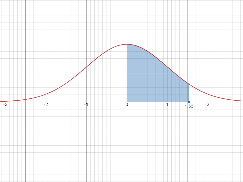
Since we’re looking for scores higher than , therefore, we’re looking for scores higher than or .

Visualizing the probability as a bell curve, we get:

We can divide this into two areas:

• The first area covers half of the curve, so it is .

• The second area covers from to , which we refer to the -table as

  Therefore, the probability that we pick a student with a test score of 30 and above is:

b) The passing score of the exam was out of questions. What is the probability that a student picked at random passed the exam?

Solution

First, we want to know how many questions did they get: this is of question which means that they should get questions right.

Now, we convert this to a -score, using the formula which gives us:

Since we want to find the probability that we get a score greater than , then we’re looking for scores higher than as well, or

Visualizing the probability as an area, we get:

We can divide this into two areas:

• The first area is half of the curve.
• Then, the second area is the region between and , which is 0.4993 from the -table
• Subtracting this yields the original probability.

Therefore,

Cheatsheet

Refer to the table below if you want to instantly know which formula to use.
Here, is the value of a score on the standard normal table.

Image	Case	Computation/Formula
		+